Tolerance Stack‑Up Analysis Basics: A Complete Guide

Here is a common engineering nightmare. A large batch of manufactured parts arrives at your facility. You inspect them carefully. Every individual component measures perfectly within its specified tolerances. Then, you begin assembly, and a critical problem emerges: the parts do not fit. A crucial gap is too small, or an alignment is off. This frustrating and costly scenario is almost always the result of a cumulative effect known as tolerance stack-up.

Tolerance stack-up analysis is a critical engineering method used to calculate the cumulative effect of part-level tolerances on a final assembly. It is a predictive tool. It determines the total possible variation in a critical dimension to ensure that components will always fit and function correctly, long before any material is cut. It is a fundamental pillar of good Design for Manufacturability (DFM).

As a manufacturing partner that emphasizes DFM, GD-Prototyping works with clients to prevent assembly issues before they arise. This guide provides a comprehensive introduction to the basics of tolerance stack-up analysis. We will explain why it is essential, how to perform a 1D analysis, and detail the two primary methods for calculating the results.

The Problem of Variation: Why Individual Tolerances Aren't Enough

To understand tolerance stack-up, one must first accept a fundamental truth of manufacturing: no two parts are ever truly identical. Every manufacturing process, from CNC machining to injection molding, has a degree of inherent, unavoidable variation. The purpose of a tolerance on an engineering drawing is to define the acceptable limits of this variation. A dimension specified as 20 mm ±0.1 mm means that any part measuring between 19.9 mm and 20.1 mm is considered a "good" part.

How Tolerances "Stack Up" in an Assembly

The problem arises when these individual, acceptable variations are combined in an assembly. Imagine stacking a pile of ten coins. Each individual coin has a small thickness tolerance. A single coin might be slightly thicker or thinner than the nominal value. When you stack ten coins together, these small, individual variations accumulate. The total height of the stack will have a much larger potential variation than any single coin. The tolerances have "stacked up."

In a mechanical assembly, this same effect occurs. The final position of a component, or the size of a critical gap, is often determined by a chain of several individual dimensions on multiple parts. Each of these dimensions has its own tolerance. The stack-up analysis is the process of summing these individual tolerances along a specific path to find the total possible variation.

The Goal of a Stack-Up Analysis

The primary goal of a stack-up analysis is to predict and manage this total variation. By performing this analysis during the design phase, an engineer can:

• Guarantee Assembly: Ensure that parts will always fit together, regardless of where they fall within their individual tolerance bands.
• Optimize Tolerances: Identify which individual part tolerances are the most critical to the assembly. This allows the engineer to tighten only the necessary tolerances, keeping manufacturing costs down.
• Reduce Rework and Scrap: Prevent the costly scenario of receiving thousands of individually "good" parts that result in "bad" assemblies.

The "How-To": Performing a 1D Tolerance Stack-Up Analysis

A one-dimensional (1D) stack-up is the most common and straightforward type of analysis. It calculates the variation along a single, linear axis. The process can be broken down into five clear steps.

A Step-by-Step Guide

Step 1: Identify the Critical Assembly Dimension First, identify the critical gap or interface that you need to control. This is the dependent variable you are trying to calculate. For example, it might be the clearance between a piston and a cylinder wall, or the alignment of two mounting holes.

Step 2: Create a Dimensional Chain (or Tolerance Path) Starting at one side of the critical dimension, trace a path through the assembly to the other side. This path must only move through the dimensions of the individual parts that directly contribute to the final assembly dimension. The path must form a closed loop, starting and ending at the two faces of the critical gap.

Step 3: List the Dimensions and Tolerances Create a simple table. In this table, list every individual part dimension that was included in the dimensional chain. Next to each dimension, list its specified tolerance from the engineering drawing.

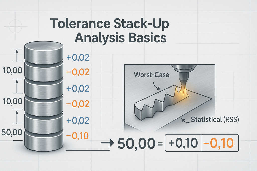
Step 4: Calculate the Total Variation This is the mathematical step. You will apply a specific method to sum the individual tolerances from your list. The two primary methods, which we will detail next, are the Worst-Case method and the Statistical (RSS) method.

Step 5: Compare the Result to the Requirement The final step is to compare your calculated total variation to the functional requirement for the assembly. For example, if your analysis shows that a critical gap can vary by ±0.5 mm, but the design requires it to be no more than ±0.2 mm, then your design has a problem. The engineer must then go back to Step 3 and strategically tighten some of the individual tolerances in the chain.

Method 1: The Worst-Case Analysis

The Worst-Case, or linear, analysis is the simplest and most conservative method for calculating tolerance stack-up. It is easy to understand and provides a definitive guarantee of assembly.

The Concept: Preparing for the Worst-Case Scenario

This method operates on a simple, powerful assumption: that all parts in the assembly have been produced at their absolute worst possible dimensional limit simultaneously. It calculates the maximum possible variation by assuming that one set of parts is at its Maximum Material Condition (MMC), and the other set is at its Least Material Condition (LMC), in a way that maximizes the final assembly error.

The Calculation

The calculation for the Worst-Case method is a simple summation. You add together the absolute values of every individual tolerance in the dimensional chain.

Total Variation (Worst-Case) = Σ (all individual tolerances)

A Detailed Worked Example

Let's analyze a simple assembly: a shaft that must fit into a housing with a specific clearance, or "gap," at the end.

• Housing Length: 50.0 mm ±0.2 mm
• Shaft Length: 49.0 mm ±0.1 mm
• The Goal: Calculate the total possible variation of the gap between the end of the shaft and the inside of the housing.

Step 1: Critical Dimension: The "Gap."

Step 2: Dimensional Chain: Start at the inside face of the housing (Face A). Move along the housing's length dimension to the outside face (Face B). Move back along the shaft's length dimension to the end of the shaft (Face C). The path is complete.

Step 3: List Dimensions:

• Housing Length: ±0.2 mm
• Shaft Length: ±0.1 mm

Step 4: Calculate the Worst

• Total Variation = (Housing Tolerance) + (Shaft Tolerance)
• Total Variation = 0.2 mm + 0.1 mm
• Total Variation = ±0.3 mm

Step 5: Compare and Interpret the Result. The nominal gap is 50.0 mm - 49.0 mm = 1.0 mm. The total variation is ±0.3 mm.

• Maximum Gap: 1.0 mm + 0.3 mm = 1.3 mm (when the housing is at its longest and the shaft is at its shortest).
• Minimum Gap: 1.0 mm - 0.3 mm = 0.7 mm (when the housing is at its shortest and the shaft is at its longest).

This analysis tells the engineer that this assembly will always have a gap between 0.7 mm and 1.3 mm. If the design can function within this range, it will work 100% of the time.

Pros and Cons of the Worst-Case Method

The main advantage of this method is that it guarantees that 100% of assemblies will fit. It is a safe and conservative approach. Its main disadvantage is that it often leads to unnecessarily tight and expensive individual part tolerances. In a complex assembly, the sum of all tolerances can become very large, forcing the engineer to specify very costly precision on each component.

Method 2: The Statistical (RSS) Analysis

The Root Sum Squared (RSS) method is a more realistic, and more complex, approach. It uses statistical principles to predict the likely variation in an assembly.

A More Realistic Approach: Root Sum Squared (RSS)

The RSS method is based on a key statistical principle: it is extremely unlikely that all parts in an assembly will be at their worst possible dimensional limit at the same time. In a stable manufacturing process, the dimensions of the parts will follow a normal distribution, or "bell curve." Most parts will be very close to the nominal dimension, and very few will be near the extreme ends of the tolerance range. The RSS method leverages this probability.

The Calculation

The calculation for the RSS method involves taking the square root of the sum of the squares of each individual tolerance.

Total Variation (RSS) = √ (Tolerance₁² + Tolerance₂² + ... + Toleranceₙ²)

The Same Worked Example, Re-calculated with RSS

Let's use the same shaft and housing assembly.

• Housing Tolerance: ±0.2 mm
• Shaft Tolerance: ±0.1 mm

Step 4: Calculate the RSS Variation.

• Total Variation = √ ( (0.2)² + (0.1)² )
• Total Variation = √ ( 0.04 + 0.01 )
• Total Variation = √ ( 0.05 )
• Total Variation = ±0.224 mm

Step 5: Compare and Interpret the Result. The RSS analysis predicts a total variation of only ±0.224 mm.

• Maximum Gap (Statistical): 1.0 mm + 0.224 mm = 1.224 mm
• Minimum Gap (Statistical): 1.0 mm - 0.224 mm = 0.776 mm

This is a much smaller range of variation than the ±0.3 mm predicted by the Worst-Case method.

Pros and Cons of the RSS Method

The main advantage of the RSS method is that it allows for more generous, less expensive individual part tolerances. It provides a more realistic prediction of the final assembly variation. The main disadvantage is that it does not guarantee 100% assembly success. The standard RSS calculation predicts the variation at ±3 standard deviations (±3σ), which corresponds to a success rate of 99.73%. This means that roughly 2,700 parts per million could fall outside the calculated range.

Choosing the Right Method and Taking Action

The choice between these two methods is a strategic decision based on the application's risk profile and production volume.

When to Use Worst-Case vs. RSS

• Use the Worst-Case method for:
  • Critical, low-volume assemblies where failure is not an option. This includes applications in aerospace, medical implants, and defense systems.
  • Assemblies with very few components, where the difference between Worst-Case and RSS is small.
  • Any situation where a 100% guarantee of fit is required.
• Use the RSS method for:
  • High-volume products, such as consumer electronics or automotive components. In these cases, it is more cost-effective to accept a statistically tiny number of out-of-spec assemblies than it is to tighten the tolerance on millions of individual parts.
  • Assemblies with a large number of components in the dimensional chain.

What to Do with the Results

If the analysis shows that the total variation is too large for the assembly to function correctly, the engineer must take action. This involves going back to the dimensional chain and strategically tightening the tolerances on one or more of the individual components. The analysis helps to identify which components have the largest impact on the stack-up, allowing the engineer to make targeted and cost-effective improvements. The choice of manufacturing process impacts the cost of tightening these tolerances. Refer to our CNC Machining Tolerances and Sheet Metal Tolerances guides for more information.

Conclusion

Tolerance stack-up analysis is an essential Design for Manufacturability (DFM) tool. It bridges the critical gap between part-level design and final assembly-level success. By predicting the cumulative effect of manufacturing variation, it allows engineers to design assemblies that fit and function correctly the first time. It is a proactive process that prevents costly redesigns, reduces scrap, and ensures a smooth transition from design to production.

Whether using the absolute safety of the Worst-Case method or the statistical realism of the RSS method, performing a stack-up analysis is a hallmark of rigorous engineering. At GD-Prototyping, our team of experts understands the critical relationship between part-level tolerances and assembly performance. We work with our clients to ensure that their designs are not only manufacturable but also ready for flawless assembly.